
developer.chat
22 September 2024
category
import numpy as np
import pandas as pd
import seaborn as sns
import matplotlib.pyplot as plt
import missingno as msno
import gc
from sklearn.model_selection import cross_val_score,GridSearchCV,train_test_split
from sklearn.tree import DecisionTreeClassifier,ExtraTreeClassifier
from sklearn.metrics import roc_curve,roc_auc_score,classification_report,mean_squared_error,accuracy_score
from sklearn.ensemble import GradientBoostingClassifier,RandomForestClassifier,BaggingClassifier,VotingClassifier,AdaBoostClassifier
In this task, you will be asked to predict the chances of a user listening to a song repetitively after the first observable listening event within a time window was triggered. If there are recurring listening event(s) triggered within a month after the user’s very first observable listening event, its target is marked 1, and 0 otherwise in the training set. The same rule applies to the testing set. KKBOX provides a training data set consists of information of the first observable listening event for each unique user-song pair within a specific time duration. Metadata of each unique user and song pair is also provided. The use of public data to increase the level of accuracy of your prediction is encouraged. The train and the test data are selected from users listening history in a given time period. Note that this time period is chosen to be before the WSDM-KKBox Churn Prediction time period. The train and test sets are split based on time, and the split of public/private are based on unique user/song pairs. Tables train.csv msno: user id song_id: song id source_system_tab: the name of the tab where the event was triggered. System tabs are used to categorize KKBOX mobile apps functions. For example, tab my library contains functions to manipulate the local storage, and tab search contains functions relating to search. source_screen_name: name of the layout a user sees. source_type: an entry point a user first plays music on mobile apps. An entry point could be album, online-playlist, song .. etc. target: this is the target variable. target=1 means there are recurring listening event(s) triggered within a month after the user’s very first observable listening event, target=0 otherwise . test.csv id: row id (will be used for submission) msno: user id song_id: song id source_system_tab: the name of the tab where the event was triggered. System tabs are used to categorize KKBOX mobile apps functions. For example, tab my library contains functions to manipulate the local storage, and tab search contains functions relating to search. source_screen_name: name of the layout a user sees. source_type: an entry point a user first plays music on mobile apps. An entry point could be album, online-playlist, song .. etc. sample_submission.csv sample submission file in the format that we expect you to submit id: same as id in test.csv target: this is the target variable. target=1 means there are recurring listening event(s) triggered within a month after the user’s very first observable listening event, target=0 otherwise . songs.csv The songs. Note that data is in unicode. song_id song_length: in ms genre_ids: genre category. Some songs have multiple genres and they are separated by | artist_name composer lyricist language members.csv user information. msno city bd: age. Note: this column has outlier values, please use your judgement. gender registered_via: registration method registration_init_time: format %Y%m%d expiration_date: format %Y%m%d song_extra_info.csv song_id song name - the name of the song. isrc - International Standard Recording Code, theoretically can be used as an identity of a song. However, what worth to note is, ISRCs generated from providers have not been officially verified; therefore the information in ISRC, such as country code and reference year, can be misleading/incorrect. Multiple songs could share one ISRC since a single recording could be re-published several times.
In [2]:
import lightgbm as lgb
from sklearn.metrics import precision_recall_curve,roc_auc_score,classification_report,roc_curve
from tqdm import tqdm
In [3]:
from subprocess import check_output

train = pd.read_csv('../input/train.csv')
test = pd.read_csv('../input/test.csv')
songs = pd.read_csv('../input/songs.csv')
members = pd.read_csv('../input/members.csv')
sample = pd.read_csv('../input/sample_submission.csv')
In [4]:
train.head()
Out[4]:
In [5]:
test.head()
Out[5]:
In [6]:
songs.head()
Out[6]:
In [7]:
members.head()
Out[7]:
In [8]:
sample.head()
members.shape
train.info()
print("\n")
songs.info()
print("\n")
members.info()
In [9]:
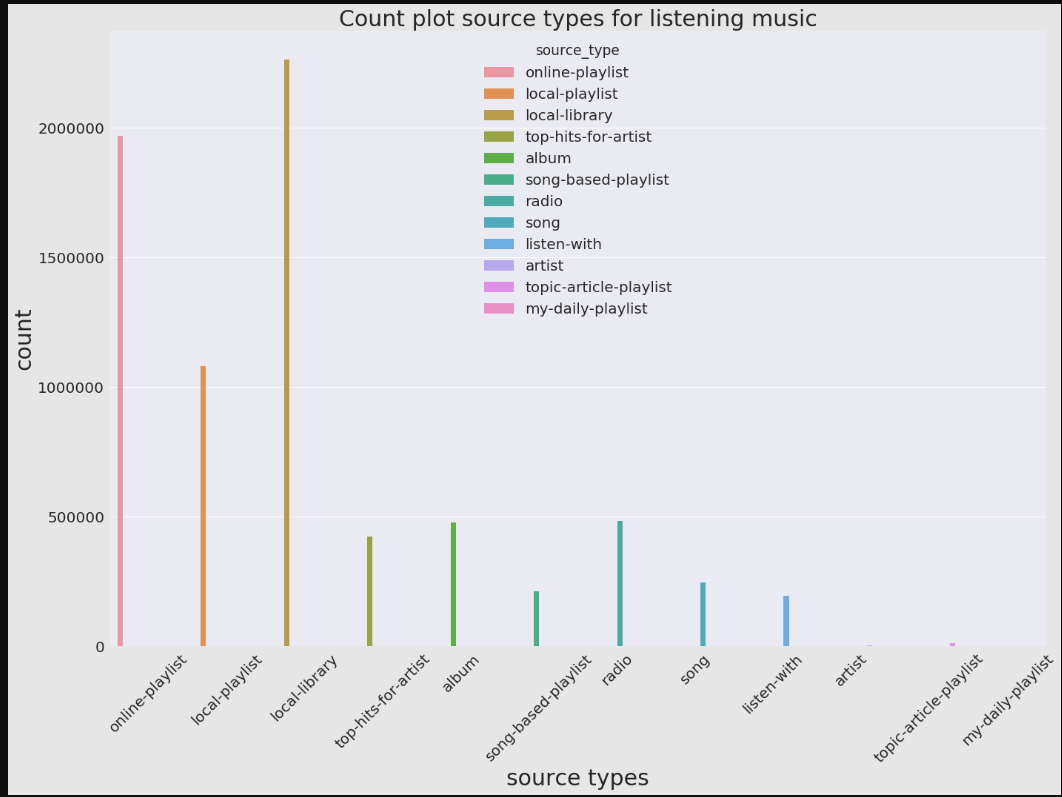
plt.figure(figsize=(20,15))
sns.set(font_scale=2)
sns.countplot(x='source_type',hue='source_type',data=train)
sns.set(style="darkgrid")
plt.xlabel('source types',fontsize=30)
plt.ylabel('count',fontsize=30)
plt.xticks(rotation='45')
plt.title('Count plot source types for listening music',fontsize=30)
plt.tight_layout()
In [10]:
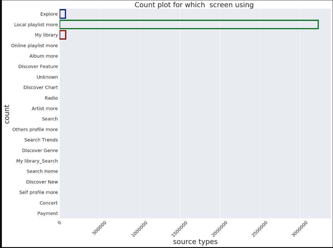
plt.figure(figsize=(20,15))
sns.set(font_scale=2)
sns.countplot(y='source_screen_name',data=train,facecolor=(0,0,0,0),linewidth=5,edgecolor=sns.color_palette('dark',3))
sns.set(style="darkgrid")
plt.xlabel('source types',fontsize=30)
plt.ylabel('count',fontsize=30)
plt.xticks(rotation='45')
plt.title('Count plot for which  screen using ',fontsize=30)
plt.tight_layout()
In [11]:
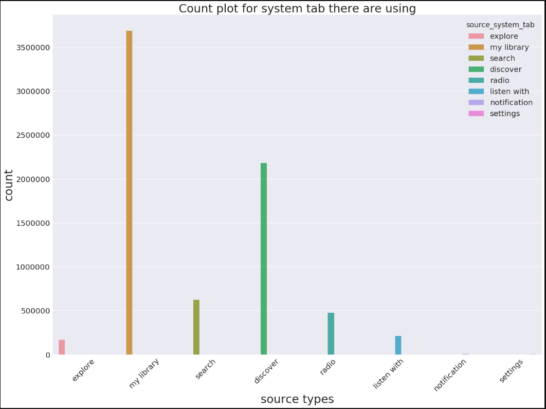
plt.figure(figsize=(20,15))
sns.set(font_scale=2)
sns.countplot(x='source_system_tab',hue='source_system_tab',data=train)
sns.set(style="darkgrid")
plt.xlabel('source types',fontsize=30)
plt.ylabel('count',fontsize=30)
plt.xticks(rotation='45')
plt.title('Count plot for system tab there are using',fontsize=30)
plt.tight_layout()
In [12]:
import matplotlib as mpl
mpl.rcParams['font.size'] = 40.0
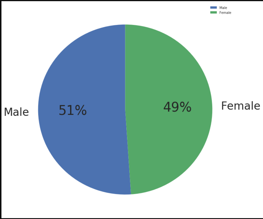
labels = ['Male','Female']
plt.figure(figsize = (12, 12))
sizes = pd.value_counts(members.gender)
patches, texts, autotexts = plt.pie(sizes,
labels=labels, autopct='%.0f%%',
shadow=False, radius=1,startangle=90)
for t in texts:
t.set_size('smaller')
plt.legend()
plt.show()
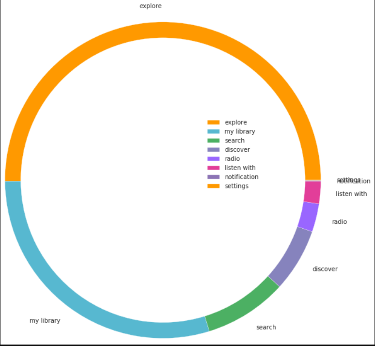
In [13]:
import matplotlib.pyplot as plt
mpl.rcParams['font.size'] = 40.0
plt.figure(figsize = (20, 20))
# Make data: I have 3 groups and 7 subgroups
group_names=['explore','my library','search','discover','radio','listen with','notification','settings']
group_size=pd.value_counts(train.source_system_tab)
print(group_size)
subgroup_names=['Male','Female']
subgroup_size=pd.value_counts(members.gender)

# Create colors
a, b, c,d,e,f,g,h=[plt.cm.autumn, plt.cm.GnBu, plt.cm.YlGn,plt.cm.Purples,plt.cm.cool,plt.cm.RdPu,plt.cm.BuPu,plt.cm.bone]

# First Ring (outside)
fig, ax = plt.subplots()
ax.axis('equal')
mypie, texts= ax.pie(group_size, radius=3.0,labels=group_names, colors=[a(0.6), b(0.6), c(0.6),d(0.6), e(0.6), f(0.6),g(0.6)])
plt.setp( mypie, width=0.3, edgecolor='white')

# Second Ring (Inside)
#mypie2, texts1 = ax.pie(subgroup_size, radius=3.0-0.3, labels=subgroup_names, labeldistance=0.7, colors=[h(0.5), b(0.4)])
#plt.setp( mypie2, width=0.3, edgecolor='white')
#plt.margins(0,0)
#for t in texts:
 #   t.set_size(25.0)
#for t in texts1:

    #t.set_size(25.0)
plt.legend()
# show it
plt.show()
In [14]:
print(members.describe())
In [15]:
print(songs.describe())
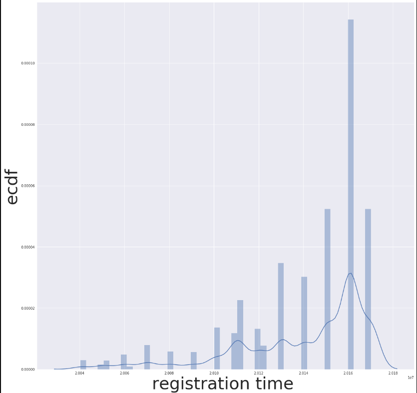
In [16]:
mpl.rcParams['font.size'] = 40.0
plt.figure(figsize = (20, 20))
sns.distplot(members.registration_init_time)
sns.set(font_scale=2)
plt.ylabel('ecdf',fontsize=50)
plt.xlabel('registration time ' ,fontsize=50)
Out[16]:
In [17]:
members.describe()
Out[17]:
In [18]:
songs.describe()
Out[18]:
In [19]:
train.describe()
Out[19]:
In [20]:
train.info()
In [21]:
members.info()
In [22]:
train_members = pd.merge(train, members, on='msno', how='inner')
train_merged = pd.merge(train_members, songs, on='song_id', how='outer')
print(train_merged.head())
In [23]:
test_members = pd.merge(test, members, on='msno', how='inner')
test_merged = pd.merge(test_members, songs, on='song_id', how='outer')
print(test_merged.head())
print(len(test_merged.columns))
In [24]:
del train_members
del test_members
In [25]:
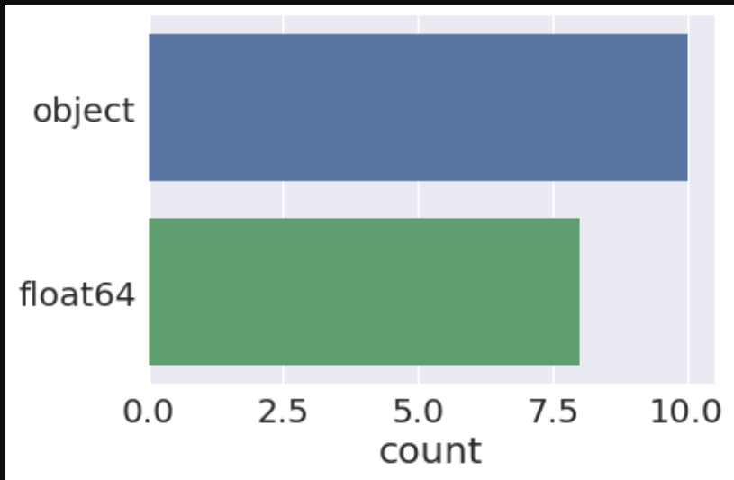
ax = sns.countplot(y=train_merged.dtypes, data=train_merged)
In [26]:
print(train_merged.columns.to_series().groupby(train_merged.dtypes).groups)
print(test_merged.columns.to_series().groupby(test_merged.dtypes).groups)
In [27]:
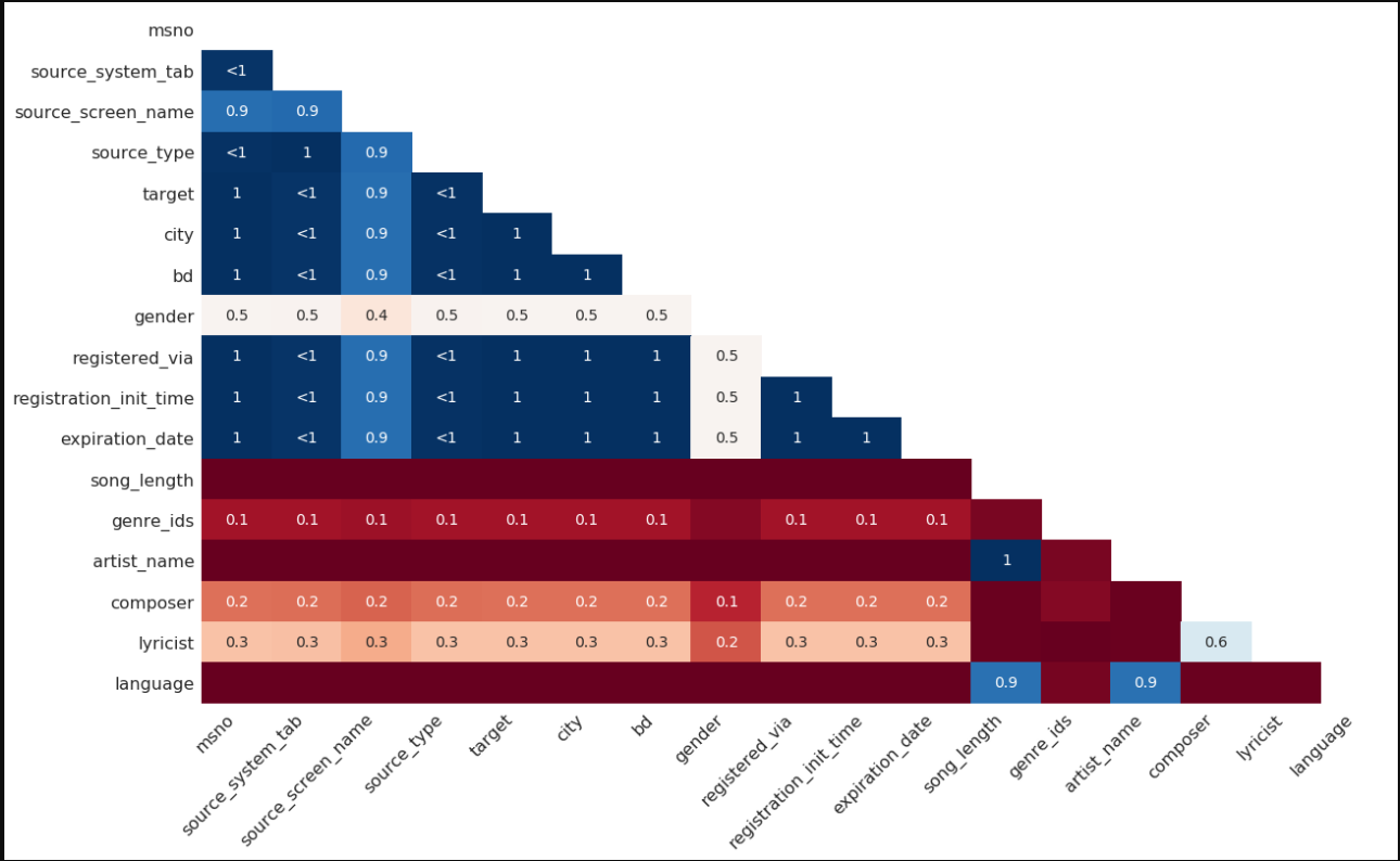
msno.heatmap(train_merged)
#msno.matrix(train_merged)
Out[27]:
In [28]:
#msno.dendrogram(train_merged)
In [29]:
#--- Function to check if missing values are present and if so print the columns having them ---
def check_missing_values(df):
    print (df.isnull().values.any())
    if (df.isnull().values.any() == True):
        columns_with_Nan = df.columns[df.isnull().any()].tolist()
    print(columns_with_Nan)
    for col in columns_with_Nan:
        print("%s : %d" % (col, df[col].isnull().sum()))

check_missing_values(train_merged)
check_missing_values(test_merged)
In [30]:
#--- Function to replace Nan values in columns of type float with -5 ---
def replace_Nan_non_object(df):
    object_cols = list(df.select_dtypes(include=['float']).columns)
    for col in object_cols:
        df[col]=df[col].fillna(np.int(-5))

replace_Nan_non_object(train_merged)
replace_Nan_non_object(test_merged)
In [31]:
#--- memory consumed by train dataframe ---
mem = train_merged.memory_usage(index=True).sum()
print("Memory consumed by training set  :   {} MB" .format(mem/ 1024**2))

#--- memory consumed by test dataframe ---
mem = test_merged.memory_usage(index=True).sum()
print("Memory consumed by test set      :   {} MB" .format(mem/ 1024**2))
In [32]:
def change_datatype(df):
    float_cols = list(df.select_dtypes(include=['float']).columns)
    for col in float_cols:
        if ((np.max(df[col]) <= 127) and(np.min(df[col] >= -128))):
            df[col] = df[col].astype(np.int8)
        elif ((np.max(df[col]) <= 32767) and(np.min(df[col] >= -32768))):
            df[col] = df[col].astype(np.int16)
        elif ((np.max(df[col]) <= 2147483647) and(np.min(df[col] >= -2147483648))):
            df[col] = df[col].astype(np.int32)
        else:
            df[col] = df[col].astype(np.int64)

change_datatype(train_merged)
change_datatype(test_merged)
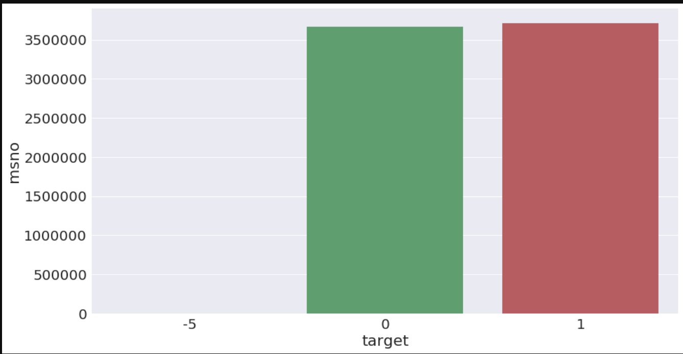
In [33]:
data = train_merged.groupby('target').aggregate({'msno':'count'}).reset_index()
a4_dims = (15, 8)
fig, ax = plt.subplots(figsize=a4_dims)
ax = sns.barplot(x='target', y='msno', data=data)
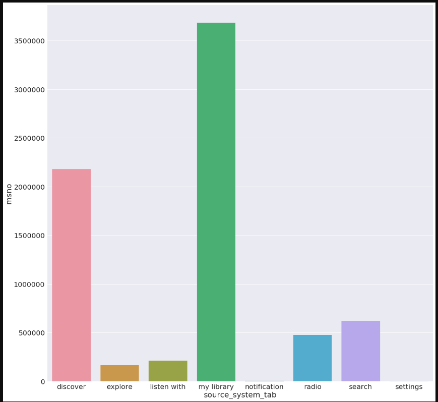
In [34]:
mpl.rcParams['font.size'] = 40.0
plt.figure(figsize = (20, 20))
data=train_merged.groupby('source_system_tab').aggregate({'msno':'count'}).reset_index()
sns.barplot(x='source_system_tab',y='msno',data=data)
Out[34]:
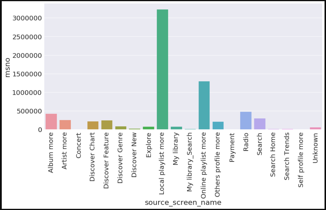
In [35]:
data = train_merged.groupby('source_screen_name').aggregate({'msno':'count'}).reset_index()
a4_dims = (15, 7)
fig, ax = plt.subplots(figsize=a4_dims)
ax = sns.barplot(x='source_screen_name', y='msno', data=data)
ax.set_xticklabels(ax.get_xticklabels(), rotation=90)
Out[35]:
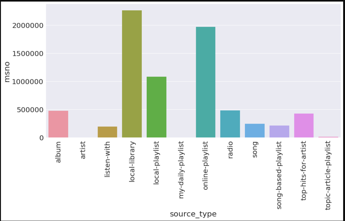
In [36]:
data = train_merged.groupby('source_type').aggregate({'msno':'count'}).reset_index()
a4_dims = (15, 7)
fig, ax = plt.subplots(figsize=a4_dims)
ax = sns.barplot(x='source_type', y='msno', data=data)
ax.set_xticklabels(ax.get_xticklabels(), rotation=90)
Out[36]:
In [37]:
data = train_merged.groupby('language').aggregate({'msno':'count'}).reset_index()
a4_dims = (15, 7)
fig, ax = plt.subplots(figsize=a4_dims)
ax = sns.barplot(x='language', y='msno', data=data)
ax.set_xticklabels(ax.get_xticklabels(), rotation=90)
Out[37]:

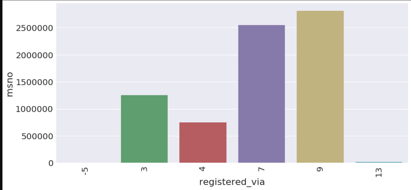
In [38]:
data = train_merged.groupby('registered_via').aggregate({'msno':'count'}).reset_index()
a4_dims = (15, 7)
fig, ax = plt.subplots(figsize=a4_dims)
ax = sns.barplot(x='registered_via', y='msno', data=data)
ax.set_xticklabels(ax.get_xticklabels(), rotation=90)
Out[38]:
In [39]:
print(train_merged.columns)
data = train_merged.groupby('city').aggregate({'msno':'count'}).reset_index()
a4_dims = (15, 7)
fig, ax = plt.subplots(figsize=a4_dims)
ax = sns.barplot(x='city', y='msno', data=data)
ax.set_xticklabels(ax.get_xticklabels(), rotation=90)
Out[39]:

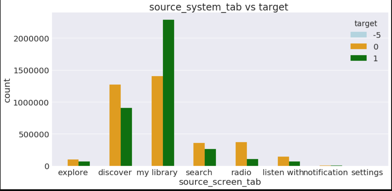
In [40]:
a4_dims = (15, 7)
fig, ax = plt.subplots(figsize=a4_dims)
ax=sns.countplot(x="source_system_tab",data=train_merged,palette=['lightblue','orange','green'],hue="target")
plt.xlabel("source_screen_tab")
plt.ylabel("count")
plt.title("source_system_tab vs target ")
plt.show()
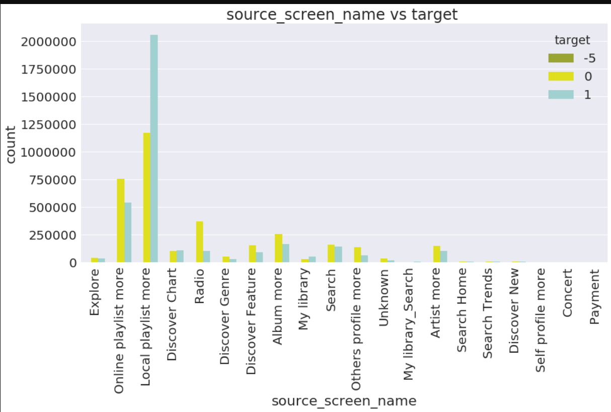
In [41]:
a4_dims = (15, 7)
fig, ax = plt.subplots(figsize=a4_dims)
ax=sns.countplot(x="source_screen_name",data=train_merged,palette=['#A8B820','yellow','#98D8D8'],hue="target")
plt.xlabel("source_screen_name")
plt.ylabel("count")
plt.title("source_screen_name vs target ")
plt.xticks(rotation='90')
plt.show()
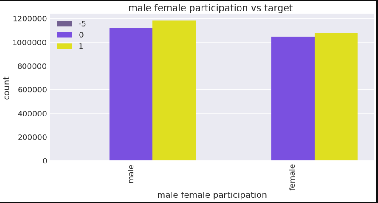
In [42]:
a4_dims = (15, 7)
fig, ax = plt.subplots(figsize=a4_dims)
ax=sns.countplot(x="gender",data=train_merged,palette=['#705898','#7038F8','yellow'],hue="target")
plt.xlabel("male female participation")
plt.ylabel("count")
plt.title("male female participation vs target ")
plt.xticks(rotation='90')
plt.legend(loc='upper left')
plt.show()
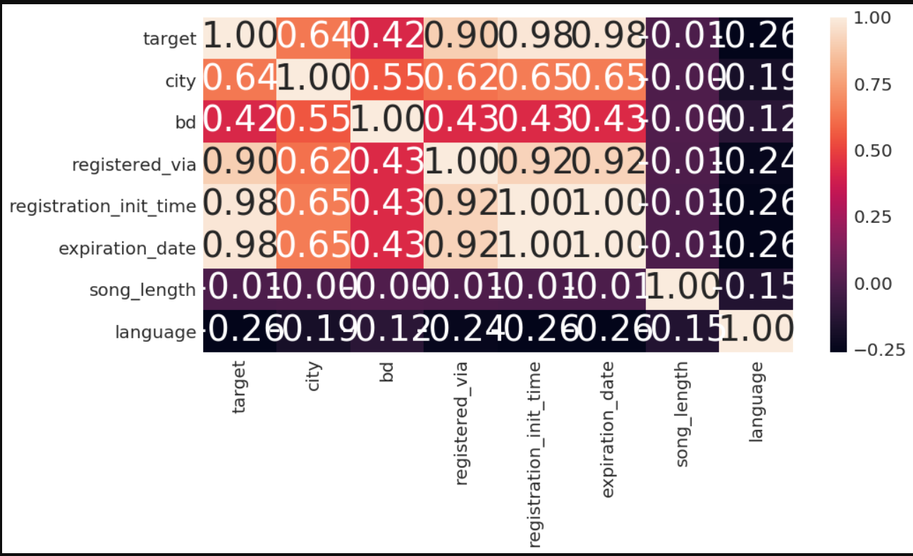
In [43]:
a4_dims = (15, 7)
fig, ax = plt.subplots(figsize=a4_dims)
ax=sns.heatmap(data=train_merged.corr(),annot=True,fmt=".2f")
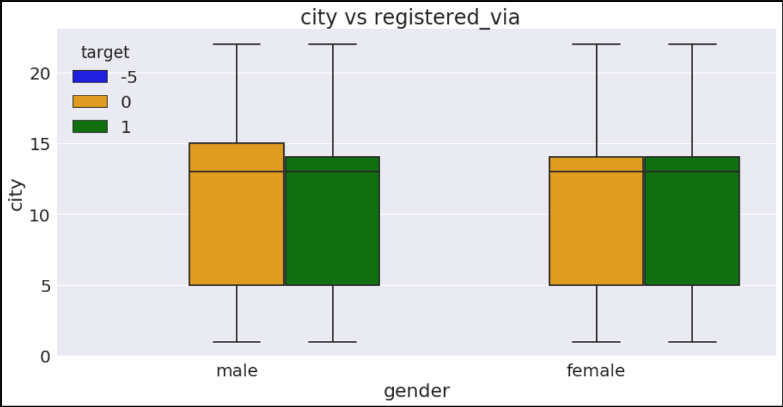
In [44]:
a4_dims = (15, 7)
fig, ax = plt.subplots(figsize=a4_dims)
ax=sns.boxplot(x="gender",y="city",data=train_merged,palette=['blue','orange','green'],hue="target")
plt.xlabel("gender")
plt.ylabel("city")
plt.title("city vs registered_via  ")
plt.show()
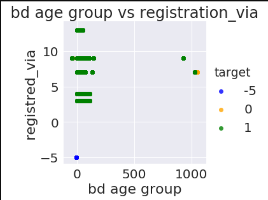
In [45]:
ax=sns.lmplot(x="bd",y="registered_via",data=train_merged,palette=['blue','orange','green'],hue="target",fit_reg=False)
plt.xlabel("bd age group")
plt.ylabel("registred_via")
plt.title(" bd age group vs registration_via ")
plt.show()
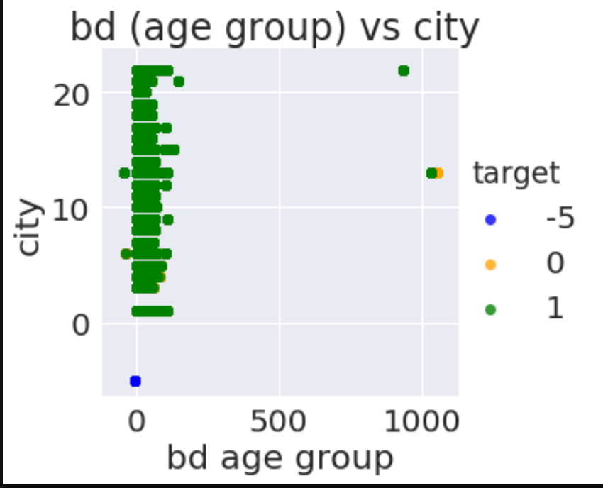
In [46]:
ax=sns.lmplot(x="bd",y="city",data=train_merged,palette=['blue','orange','green'],hue="target",fit_reg=False)
plt.xlabel("bd age group")
plt.ylabel("city")
plt.title("bd (age group) vs city ")
plt.show()
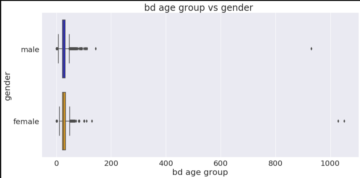
In [47]:
#remomving outlier from bd age group column
In [48]:
a4_dims = (15, 7)
fig, ax = plt.subplots(figsize=a4_dims)
ax=sns.boxplot(x="bd",y="gender",data=train_merged,palette=['blue','orange','green'])
plt.xlabel("bd age group")
plt.ylabel("gender")
plt.title("bd age group vs gender ")
plt.show()
In [49]:
train_merged.describe()
def remove_outlier(df_in, col_name):

    #q1 = df_in[col_name].quantile(0.25)
    #q3 = df_in[col_name].quantile(0.75)
    #iqr = q3-q1 #Interquartile range
    fence_low  = 12
    fence_high = 45
    df_out = df_in.loc[(df_in[col_name] > fence_low) & (df_in[col_name] < fence_high)]
    return df_out
df_final_train=remove_outlier(train_merged,'bd')
In [50]:
# This Python 3 environment comes with many helpful analytics libraries installed
# It is defined by the kaggle/python docker image: https://github.com/kaggle/docker-python
# For example, here's several helpful packages to load in

import numpy as np # linear algebra
import pandas as pd # data processing, CSV file I/O (e.g. pd.read_csv)
import lightgbm as lgb

# Input data files are available in the "../input/" directory.
# For example, running this (by clicking run or pressing Shift+Enter) will list the files in the input directory

from subprocess import check_output
print(check_output(["ls", "../input"]).decode("utf8"))

# Any results you write to the current directory are saved as output.
In [51]:
print('Loading data...')
data_path = '../input/'
train = pd.read_csv(data_path + 'train.csv', dtype={'msno' : 'category',
                                                'source_system_tab' : 'category',
                                                  'source_screen_name' : 'category',
                                                  'source_type' : 'category',
                                                  'target' : np.uint8,
                                                  'song_id' : 'category'})
test = pd.read_csv(data_path + 'test.csv', dtype={'msno' : 'category',
                                                'source_system_tab' : 'category',
                                                'source_screen_name' : 'category',
                                                'source_type' : 'category',
                                                'song_id' : 'category'})
songs = pd.read_csv(data_path + 'songs.csv',dtype={'genre_ids': 'category',
                                                  'language' : 'category',
                                                  'artist_name' : 'category',
                                                  'composer' : 'category',
                                                  'lyricist' : 'category',
                                                  'song_id' : 'category'})
members = pd.read_csv(data_path + 'members.csv',dtype={'city' : 'category',
                                                      'bd' : np.uint8,
                                                      'gender' : 'category',
                                                      'registered_via' : 'category'},
                     parse_dates=['registration_init_time','expiration_date'])
songs_extra = pd.read_csv(data_path + 'song_extra_info.csv')
print('Done loading...')
In [52]:
song_cols = ['song_id', 'artist_name', 'genre_ids', 'song_length', 'language']
train = train.merge(songs[song_cols], on='song_id', how='left')
test = test.merge(songs[song_cols], on='song_id', how='left')

members['registration_year'] = members['registration_init_time'].apply(lambda x: int(str(x)[0:4]))
#members['registration_month'] = members['registration_init_time'].apply(lambda x: int(str(x)[4:6]))
#members['registration_date'] = members['registration_init_time'].apply(lambda x: int(str(x)[6:8]))

members['expiration_year'] = members['expiration_date'].apply(lambda x: int(str(x)[0:4]))
members['expiration_month'] = members['expiration_date'].apply(lambda x: int(str(x)[4:6]))
#members['expiration_date'] = members['expiration_date'].apply(lambda x: int(str(x)[6:8]))

# exepting some unimportanat features


# Convert date to number of days
members['membership_days'] = (members['expiration_date'] - members['registration_init_time']).dt.days.astype(int)

#members = members.drop(['registration_init_time'], axis=1)
#members = members.drop(['expiration_date'], axis=1)
In [53]:
# categorize membership_days
members['membership_days'] = members['membership_days']//200
members['membership_days'] = members['membership_days'].astype('category')
In [54]:
member_cols = ['msno','city','registered_via', 'registration_year', 'expiration_year', 'membership_days']

train = train.merge(members[member_cols], on='msno', how='left')
test = test.merge(members[member_cols], on='msno', how='left')
In [55]:
train.info()
In [56]:
def isrc_to_year(isrc):
    if type(isrc) == str:
        if int(isrc[5:7]) > 17:
            return int(isrc[5:7])//5
        else:
            return int(isrc[5:7])//5
    else:
        return np.nan
#categorize song_year per 5years

songs_extra['song_year'] = songs_extra['isrc'].apply(isrc_to_year)
songs_extra.drop(['isrc', 'name'], axis = 1, inplace = True)
In [57]:
train = train.merge(songs_extra, on = 'song_id', how = 'left')
test = test.merge(songs_extra, on = 'song_id', how = 'left')
In [58]:
train['genre_ids'] = train['genre_ids'].str.split('|').str[0]
In [59]:
temp_song_length = train['song_length']
In [60]:
train.drop('song_length', axis = 1, inplace = True)
test.drop('song_length',axis = 1 , inplace =True)
In [61]:
train.head()
Out[61]:
In [62]:
song_count = train.loc[:,["song_id","target"]]

# measure repeat count by played songs
song_count1 = song_count.groupby(["song_id"],as_index=False).sum().rename(columns={"target":"repeat_count"})

# count play count by songs
song_count2 = song_count.groupby(["song_id"],as_index=False).count().rename(columns = {"target":"play_count"})
In [63]:
song_repeat = song_count1.merge(song_count2,how="inner",on="song_id")
song_repeat["repeat_percentage"] = round((song_repeat['repeat_count']*100) / song_repeat['play_count'],1)
song_repeat['repeat_count'] = song_repeat['repeat_count'].astype('int')
song_repeat['repeat_percentage'] = song_repeat['repeat_percentage'].replace(100.0,np.nan)
#cuz most of 100.0 are played=1 repeated=1 values. I think it is not fair compare with other played a lot songs
In [64]:
train = train.merge(song_repeat,on="song_id",how="left")
test = test.merge(song_repeat,on="song_id",how="left")
In [65]:
# type cast
test['song_id'] = test['song_id'].astype('category')
test['repeat_count'] = test['repeat_count'].fillna(0)
test['repeat_count'] = test['repeat_count'].astype('int')
test['play_count'] = test['play_count'].fillna(0)
test['play_count'] = test['play_count'].astype('int')
#train['repeat_percentage'].replace(100.0,np.nan)
In [66]:
artist_count = train.loc[:,["artist_name","target"]]

# measure repeat count by played songs
artist_count1 = artist_count.groupby(["artist_name"],as_index=False).sum().rename(columns={"target":"repeat_count_artist"})

# measure play count by songs
artist_count2 = artist_count.groupby(["artist_name"],as_index=False).count().rename(columns = {"target":"play_count_artist"})

artist_repeat = artist_count1.merge(artist_count2,how="inner",on="artist_name")
In [67]:
artist_repeat["repeat_percentage_artist"] = round((artist_repeat['repeat_count_artist']*100) / artist_repeat['play_count_artist'],1)
artist_repeat['repeat_count_artist'] = artist_repeat['repeat_count_artist'].fillna(0)
artist_repeat['repeat_count_artist'] = artist_repeat['repeat_count_artist'].astype('int')
artist_repeat['repeat_percentage_artist'] = artist_repeat['repeat_percentage_artist'].replace(100.0,np.nan)
In [68]:
#use only repeat_percentage_artist
del artist_repeat['repeat_count_artist']
#del artist_repeat['play_count_artist']
In [69]:
#merge it with artist_name to train dataframe
train = train.merge(artist_repeat,on="artist_name",how="left")
test = test.merge(artist_repeat,on="artist_name",how="left")
In [70]:
train.info()
In [71]:
del train['artist_name']
del test['artist_name']
In [72]:
msno_count = train.loc[:,["msno","target"]]

# count repeat count by played songs
msno_count1 = msno_count.groupby(["msno"],as_index=False).sum().rename(columns={"target":"repeat_count_msno"})

# count play count by songs
msno_count2 = msno_count.groupby(["msno"],as_index=False).count().rename(columns = {"target":"play_count_msno"})

msno_repeat = msno_count1.merge(msno_count2,how="inner",on="msno")
In [73]:
msno_repeat["repeat_percentage_msno"] = round((msno_repeat['repeat_count_msno']*100) / msno_repeat['play_count_msno'],1)
msno_repeat['repeat_count_msno'] = msno_repeat['repeat_count_msno'].fillna(0)
msno_repeat['repeat_count_msno'] = msno_repeat['repeat_count_msno'].astype('int')
#msno_repeat['repeat_percentage_msno'] = msno_repeat['repeat_percentage_msno'].replace(100.0,np.nan)
# it can be meaningful so do not erase 100.0
In [74]:
#merge it with msno to train dataframe
train = train.merge(msno_repeat,on="msno",how="left")
test = test.merge(msno_repeat,on="msno",how="left")
In [75]:
import gc
#del members, songs; gc.collect();

for col in train.columns:
    if train[col].dtype == object:
        train[col] = train[col].astype('category')
        test[col] = test[col].astype('category')
In [76]:
train['song_year'] = train['song_year'].astype('category')
test['song_year'] = test['song_year'].astype('category')
In [77]:
train.head()
Out[77]:
In [78]:
drop_list = ['repeat_count','repeat_percentage',
             'repeat_percentage_artist',
             'repeat_count_msno','repeat_percentage_msno'
            ]
train = train.drop(drop_list,axis=1)
test = test.drop(drop_list,axis=1)
In [79]:
test['play_count_msno'] = test['play_count_msno'].fillna(0)
test['play_count_msno'] = test['play_count_msno'].astype('int')


train['play_count_artist'] = train['play_count_artist'].fillna(0)
test['play_count_artist'] = test['play_count_artist'].fillna(0)
train['play_count_artist'] = train['play_count_artist'].astype('int')
test['play_count_artist'] = test['play_count_artist'].astype('int')
In [80]:
from sklearn.model_selection import KFold
# Create a Cross Validation with 3 splits
kf = KFold(n_splits=3)

predictions = np.zeros(shape=[len(test)])

# For each KFold
for train_indices ,validate_indices in kf.split(train) :
    train_data = lgb.Dataset(train.drop(['target'],axis=1).loc[train_indices,:],label=train.loc[train_indices,'target'])
    val_data = lgb.Dataset(train.drop(['target'],axis=1).loc[validate_indices,:],label=train.loc[validate_indices,'target'])

    params = {
            'objective': 'binary',
            'boosting': 'gbdt',
            'learning_rate': 0.2 ,
            'verbose': 0,
            'num_leaves': 2**8,
            'bagging_fraction': 0.95,
            'bagging_freq': 1,
            'bagging_seed': 1,
            'feature_fraction': 0.9,
            'feature_fraction_seed': 1,
            'max_bin': 256,
            'num_rounds': 80,
            'metric' : 'auc'
        }
    # Train the model
    lgbm_model = lgb.train(params, train_data, 100, valid_sets=[val_data])
    predictions += lgbm_model.predict(test.drop(['id'],axis=1))
    del lgbm_model
    # We get the ammount of predictions from the prediction list, by dividing the predictions by the number of Kfolds.
predictions = predictions/3

INPUT_DATA_PATH = '../input/'

# Read the sample_submission CSV
submission = pd.read_csv(INPUT_DATA_PATH + '/sample_submission.csv')
# Set the target to our predictions
submission.target=predictions
# Save the submission file
submission.to_csv('submission.csv',index=False)
引用
- 登录 发表评论